CALIFORNIA PM2.5
PREDICTION MODEL
Our flagship model demonstrates what we can build for your organization. Daily PM2.5 predictions across 129 California monitoring stations, powered by NASA/NOAA satellite data and LightGBM machine learning.
What This Model Does
The California PM2.5 model predicts fine particulate matter concentrations and breaks them down into their chemical components. This enables understanding of pollution sources and health impacts beyond simple mass measurements.
- LightGBM gradient boosting with Bayesian optimization
- Purged K-fold cross-validation with 30-day gap
- 16.7% improvement over Elastic Net baseline
- Robust to temporal autocorrelation
- Validated against EPA ground monitoring
From Raw Data to Predictions
A rigorous data science pipeline ensuring quality and reproducibility at every step.
Data Collection
Ingested 81,197 daily observations from 147 EPA stations across California, merged with HRRR meteorological data, GEOS-CF atmospheric composition, and MAIAC satellite AOD.
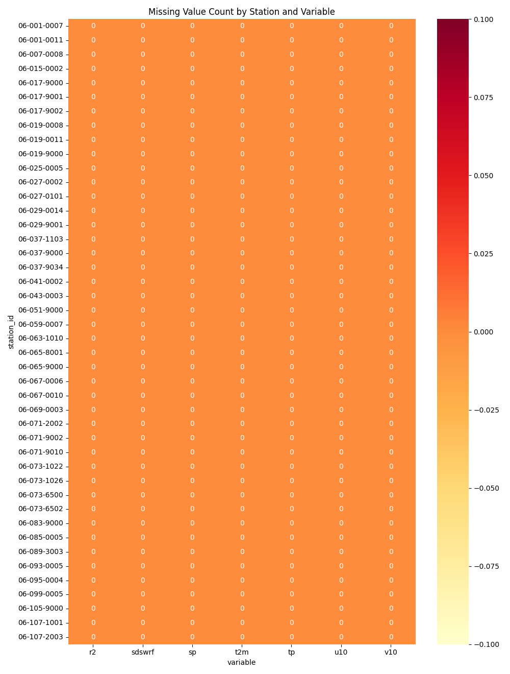
Data Cleaning
Dropped EPA speciated columns (94% missing), removed MAIAC water vapor (38% missing), and filtered incomplete rows. Retained complete cases only to maintain data quality.
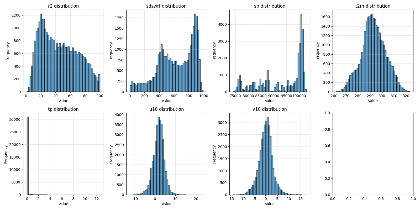
Exploratory Analysis
Analyzed feature distributions, temporal patterns, and correlations. HRRR variables show expected meteorological patterns; MAIAC AOD captures aerosol loading variability.
Model Training
Trained LightGBM with Bayesian hyperparameter optimization. Used Purged K-Fold CV with 30-day temporal gap to prevent data leakage from autocorrelation.
Exploratory Data Analysis
Before training any model, we conducted rigorous statistical analysis to understand data distributions, feature relationships, and spatio-temporal patterns. Here are the key findings.
Target Variable Distribution (PM2.5)
Key Finding: PM2.5 distribution is right-skewed (skewness = 2.14), with most days showing good air quality but occasional high-pollution events reaching 98.2 µg/m³. This suggests the model must handle both typical conditions and extreme events.
EPA AQI Category Distribution
Feature-Target Correlations
Top Predictive Features
Correlation Insights
GEOS-CF PM2.5 shows the strongest correlation (r=0.42), validating that the NASA atmospheric model captures real PM2.5 variability.
MAIAC AOD features (r≈0.30) confirm satellite-derived aerosol optical depth as a strong PM2.5 proxy, consistent with peer-reviewed literature.
Temperature shows negative correlation (r=-0.14), indicating higher PM2.5 in cooler conditions—likely due to winter inversions and heating emissions.
Multicollinearity Check
maiac_AOD_047 ↔ maiac_AOD_055: r=0.97 — Expected - same instrument. Handled via tree-based model's implicit feature selection.
Seasonal Patterns
Winter shows 52% higher PM2.5 than Spring, driven by atmospheric inversions and residential heating.
Spatial Variation
Highest PM2.5 Stations
Lowest PM2.5 Stations
Central Valley stations show 3-4x higher PM2.5 than coastal sites—topographic basin trapping is a key factor.
EDA-Driven Model Design
Our exploratory analysis directly informed model architecture: the right-skewed target distribution guided our choice of tree-based methods over linear models; high multicollinearity between AOD bands validated LightGBM's implicit feature selection; and strong seasonal patterns justified temporal cross-validation with 30-day purging gaps to prevent data leakage.
Key Input Features
The model combines satellite observations with meteorological data to predict ground-level PM2.5 concentrations.
Aerosol Optical Depth
MAIAC satellite aerosol loading
Temperature
HRRR 2m air temperature
Relative Humidity
HRRR atmospheric moisture
Wind Speed
HRRR u/v wind components
GEOS PM2.5
NASA GEOS-CF model estimate
Nitrogen Dioxide
GEOS-CF trace gas
Data Sources
The model fuses data from multiple satellite and ground-based sources to create comprehensive feature sets for prediction.
GEOS-CF
Global atmospheric composition forecasts providing chemical concentrations and meteorological variables.
HRRR
High-Resolution Rapid Refresh model for detailed meteorological conditions.
MAIAC
Multi-Angle Implementation of Atmospheric Correction for satellite aerosol optical depth.
CSN
Chemical Speciation Network ground truth measurements for model training and validation.
Research Foundation
Methodology grounded in peer-reviewed research
Spatial+: A new cross-validation method to evaluate geospatial machine learning models
Wang, Y., Khodadadzadeh, M., & Zurita-Milla, R.
Foundation for unbiased cross-validation of spatio-temporal models for species distribution modeling
Koldasbayeva, D., & Zaytsev, A.
Spatiotemporal prediction of continuous daily PM2.5 concentrations across China using a spatially explicit machine learning algorithm
Zhan, Y., Luo, Y., Deng, X., Chen, H., Grieneisen, M. L., et al.
Comparison of different missing-imputation methods for MAIAC AOD in estimating daily PM2.5 levels
Chen, Z.-Y., Jin, J.-Q., Zhang, R., Zhang, T.-H., et al.
Autocorrelation in Earth and Planetary Sciences
Elsevier
Want Something Similar?
We can build a custom environmental prediction model for your region, variables, and use case. Let's discuss your requirements.